Classify Titanic passangers

In this example, I would like to show you how to analyze Titanic dataset with AutoML mljar-supervised. The AutoML will do all the job and let's go through all results.

All the code and results are available at the GitHub

The code

What does python code do:

• reads Titanic train dataset (the same data as in Kaggle platform),
• trains AutoML object,
• computes predictions and accuracy on test dataset (the same test data as in Kaggle)

import pandas as pd
import numpy as np
from sklearn.metrics import accuracy_score
from supervised import AutoML

train = pd.read_csv("https://raw.githubusercontent.com/pplonski/datasets-for-start/master/Titanic/train.csv")

X = train[train.columns[2:]]
y = train["Survived"]

automl = AutoML(results_path="AutoML_3")
automl.fit(X, y)

test = pd.read_csv("https://raw.githubusercontent.com/pplonski/datasets-for-start/master/Titanic/test_with_Survived.csv")
predictions = automl.predict(test)
print(f"Accuracy: {accuracy_score(test['Survived'], predictions)*100.0:.2f}%" )

As you see from above example the heavy job is done in exactly 2 lines of code:

automl = AutoML(results_path="AutoML_3")
automl.fit(X, y)

I will show you step by step what above code produced based on the training data.

The Explain mode

The default mode for mljar-supervised is Explain, which means that:

• there will be used 75% / 25% for train / test split for model training and evaluation,
• there will be trained following algorithms: Baseline, Decision Tree, Linear, Random Forest, Xgboost, Neural Network, and Ensemble,
• the full explanations will be created.

All results created during AutoML training will be saved to the hard drive. There will be Markdown report in the README.md file for each model available (no black-boxes!).

The AutoML leaderboard report

The main README.md in the report will contain:

• table will all models performance,
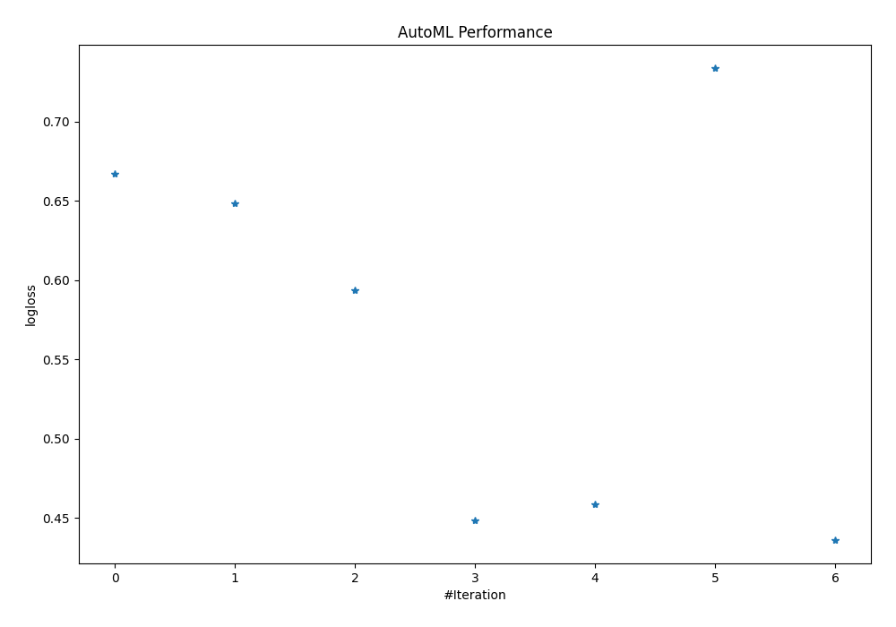
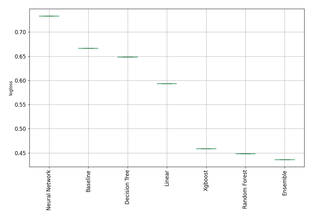
• performance plotted as scatter plot and box plot.

The leaderbord:

Best model	name	model_type	metric_type	metric_value	train_time	Link
	1_Baseline	Baseline	logloss	0.666775	0.26	Results link
	2_DecisionTree	Decision Tree	logloss	0.648504	18	Results link
	3_Linear	Linear	logloss	0.593649	12.2	Results link
	4_Default_RandomForest	Random Forest	logloss	0.448691	22.24	Results link
	5_Default_Xgboost	Xgboost	logloss	0.458922	12.63	Results link
	6_Default_NeuralNetwork	Neural Network	logloss	0.733411	23.84	Results link
the best	Ensemble	Ensemble	logloss	0.436319	0.83	Results link

From the above table you can check what was the performance of the models and how long was the training. There is a Results link in the table for each model (please scroll this table if you don't see it), which you can click and go into model details

The performance is presented in the plots:

The Baseline

The Baseline algorithm is very important during initial analysis. It tells us about quality of our data and helps to check if we need Machine Learning to solve this problem.

Let's compute the percentage difference between the best model (Ensemble) and the Baseline:

% difference = (0.667 - 0.436) / 0.667 * 100.0 = 34.6% 

The best model is 34.6% better than Baseline, the usage of ML is justifed and the data doesn't look like the random data.

When data looks like random?

I personally assume that if the best model is less than 5% better than Baseline then data looks like the random data and ML usage should be reconsidered.

Decision Tree

Let's look closer into Decision Tree report.

The part of report is below:

Decision Tree hyperparameters

• criterion: gini
• max_depth: 3
• explain_level: 2

Validation

• validation_type: split
• train_ratio: 0.75
• shuffle: True
• stratify: True

Optimized metric

logloss

Training time

17.1 seconds

Metric details

	score	threshold
logloss	0.648504	nan
auc	0.814293	nan
f1	0.728261	0.351143
accuracy	0.775785	0.351143
precision	0.843137	0.597938
recall	0.965116	0
mcc	0.54213	0.351143

Confusion matrix (at threshold=0.351143)

	Predicted as negative	Predicted as positive
Labeled as negative	106	31
Labeled as positive	19	67

There are many metrics and confusion matrix pre-computed.

Additionally, there is a Decision Tree visualization:

There are created many explanations for each model. Let's check how they look like for Xgboost (the best single model).

The Xgboost model

You can check details of Xgboost model in the Markdown report. Here I will show some parts of the report with short comment.

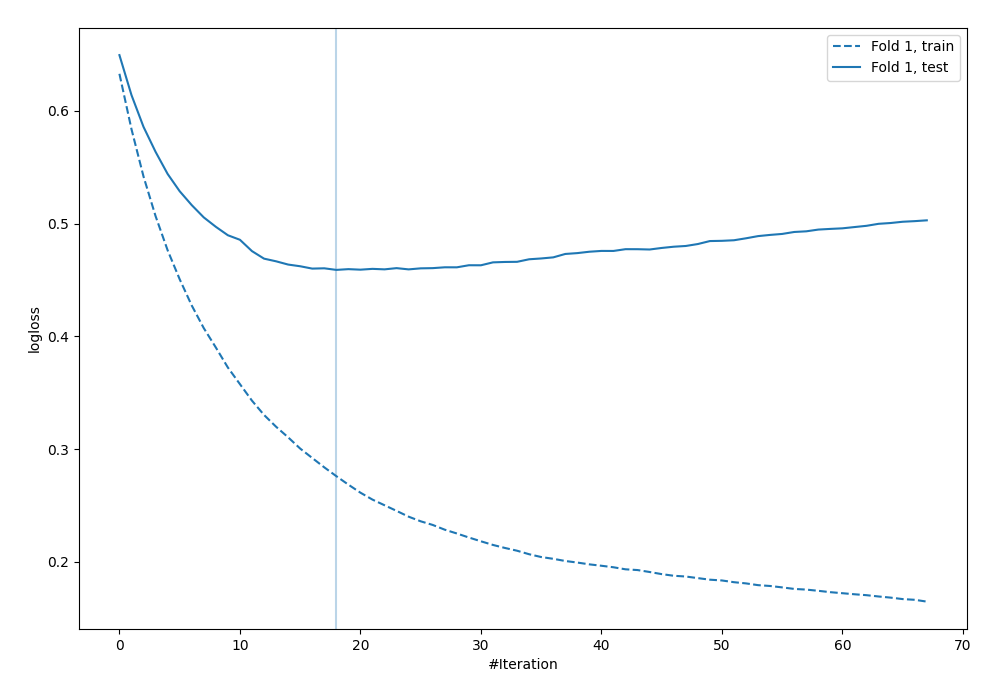
Learning curves

The vertical line indicates the optimal number of trees in the Xgboost (found with early stopping). This number of trees will be used during computning predictions.

Feature Importance

The permutation-based feature importance:

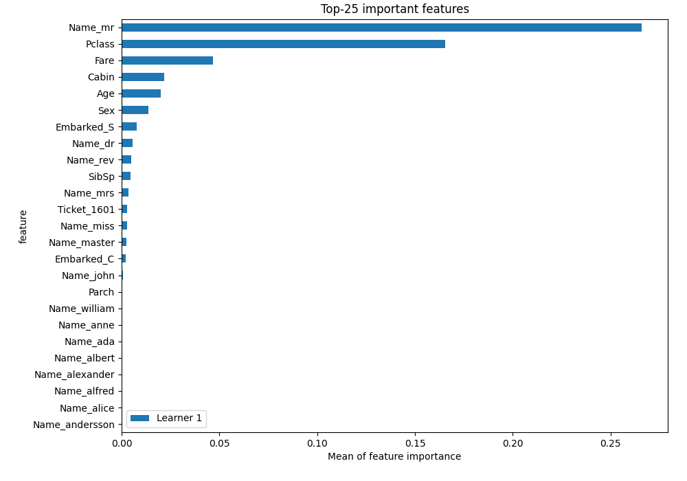
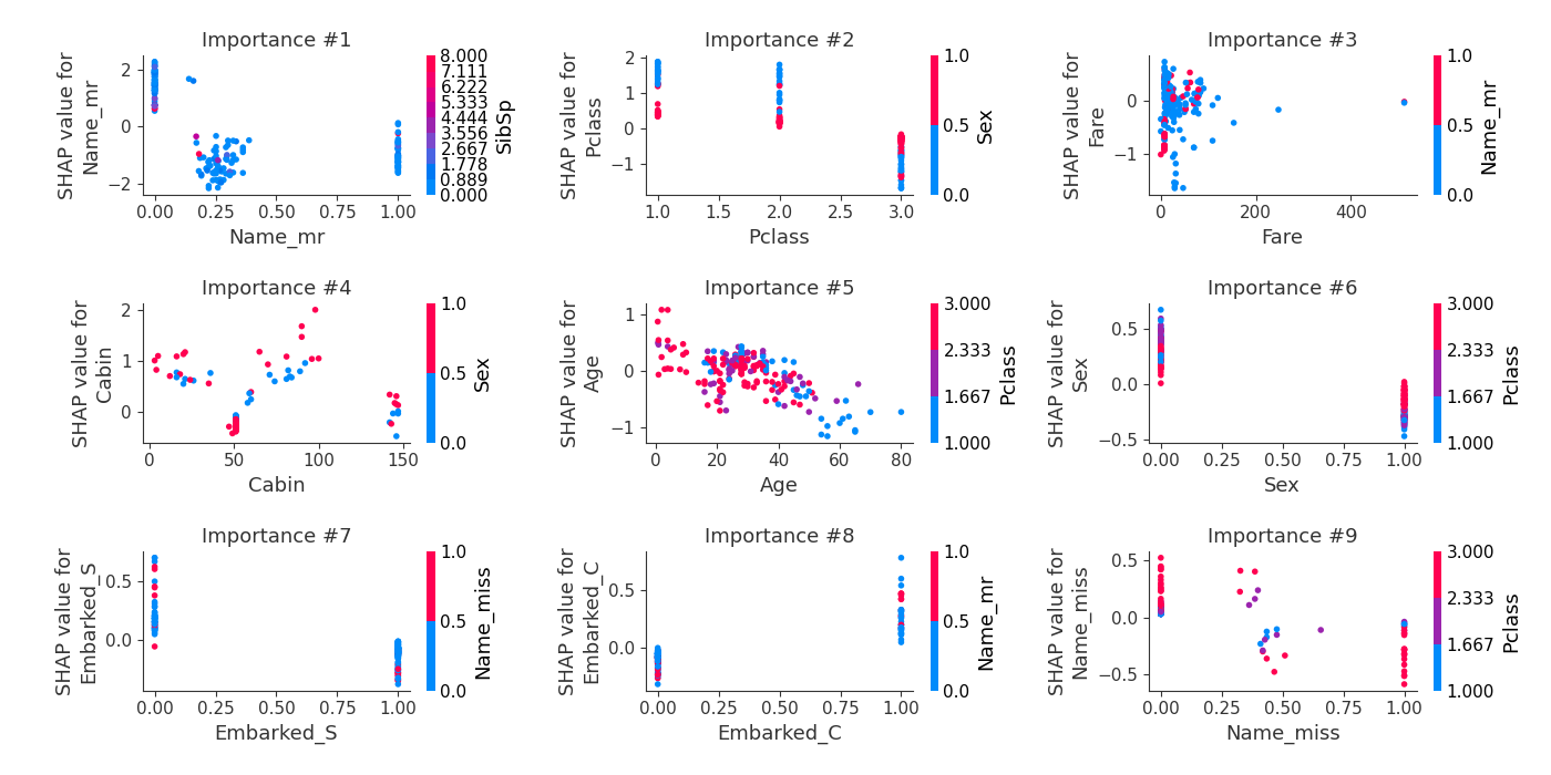
From the plot you can see that the most used feature is Name_mr. There wasn't such feature in the training data. There was Name feature. The AutoML used TF-IDF transformation (scikit-learn TfidfVectorizer) to construct new features from Name text feature.

SHAP dependence plots

The test accuracy

The AutoML is used to predict the labels for test data samples. The accuracy computed on test data:

AutoML directory: AutoML_3
The task is binary_classification with evaluation metric logloss
AutoML will use algorithms: ['Baseline', 'Linear', 'Decision Tree', 'Random Forest', 'Xgboost', 'Neural Network']
AutoML will ensemble availabe models
AutoML steps: ['simple_algorithms', 'default_algorithms', 'ensemble']
* Step simple_algorithms will try to check up to 3 models
1_Baseline logloss 0.666775 trained in 0.23 seconds
2_DecisionTree logloss 0.648504 trained in 17.06 seconds
3_Linear logloss 0.593649 trained in 11.04 seconds
* Step default_algorithms will try to check up to 3 models
4_Default_RandomForest logloss 0.448691 trained in 21.72 seconds
5_Default_Xgboost logloss 0.458922 trained in 17.47 seconds
6_Default_NeuralNetwork logloss 0.718124 trained in 22.08 seconds
* Step ensemble will try to check up to 1 model
Ensemble logloss 0.436478 trained in 0.71 seconds
AutoML fit time: 96.77 seconds
Accuracy: 77.99%

Summary

The AutoML was used to analyze Titanic dataset. I hope you see advantages of AutoML (with 2 lines of code):

• all needed preprocessing were done automatically: insert missing values, convert categoricals, convert text to numbers.
• there were checked many different algorithms,
• all results are saved to the hard drive, Markdown reports are available for all models.

Do you see If you are still asking yourself if AutoML will replace data scientist. Then I hope you have an answer now. Yes, the AutoML will replace Data Scientists who are not using AutoML with the ones that are using AutoML.